Lid Driven Cavity Flow
Configuration
1. We want to have a lid driven cavity flow with (according to the QPF) :
Small Reynolds Number
Re = 0.000061
dom = DomainRectFluid(nu_=1.0, dimx=0.82, dimy=0.61, delta_x=0.02)
vel = 0.0001

cfd_lid_driven(10, 0.30)
2. Works also with another configuration to get another Reynolds number :
High Reynolds Number
Re = 300
size = 1.0
dom = DomainRectFluid(dimx=size, dimy=size, delta_x=size / 60, rho=1.0, nu_=0.01)

vel = 3.0
Because we are at high Reynolds number :
we need to have an important t_end
Moreover to avoid the following error:
RuntimeError: too many sub iterations 10101
one can put more saving moments to have weaker iterations.
Reference case
the script
	"""Example on how to solve a Lid driven cavity problem with the navier stokes solver"""

	from barbatruc.fluid_domain import DomainRectFluid
	from barbatruc.fd_ns_2d import NS_fd_2D_explicit

	# from barbatruc.lattice import Lattice

	__all__ = ["cfd_lid_driven"]


	# pylint: disable=duplicate-code
	def cfd_lid_driven(nsave, tchar):
	    """Startup computation
	    solve a lid_driven_cavity  problem
	    """
	    size = 1.0
	    dom = DomainRectFluid(dimx=size, dimy=size, delta_x=size / 60, rho=1.0, nu_=0.01)

	    vel = 3.0
	    t_end = tchar * size / vel
	    dom.switch_bc_xmin_wall_noslip()
	    dom.switch_bc_xmax_wall_noslip()
	    dom.switch_bc_ymax_moving_wall(vel_u=vel)
	    dom.switch_bc_ymin_wall_noslip()

	    time = 0.0
	    time_step = t_end / nsave

	    # solver = Lattice(dom, max_vel=2*vel)
	    solver = NS_fd_2D_explicit(
	        dom, obs_ib_factor=0.01, press_maxsteps=200, press_tol=5.0e-3, max_vel=4.0
	    )
	    for i in range(nsave):
	        time += time_step
	        solver.iteration(time, time_step)
	        print("\n\n===============================")
	        print(f"\n  Iteration {i+1}/{nsave}, Time :, {time}s")
	        print(f"  Reynolds : {dom.reynolds(size)}")
	        print(dom.fields_stats())
	        dom.dump_paraview(time=time)
	        dom.dump_global(time=time)
	    dom.show_fields()
	    dom.show_flow()
	    dom.show_profile_y(xtgt=0.41)
	    print("Normal end of execution.")


	if __name__ == "__main__":
	    cfd_lid_driven(10, 10)
For Re = 0.000061
The flow output :
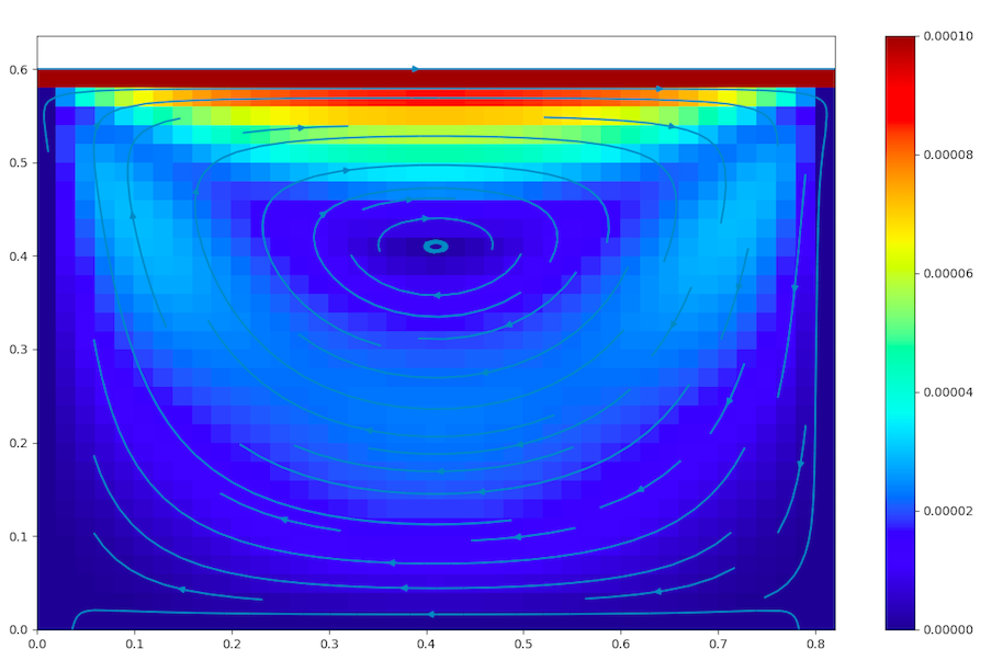 cavityflow
The fields :
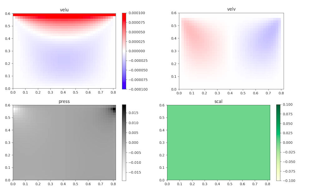 cavityfields
The velocity profile :
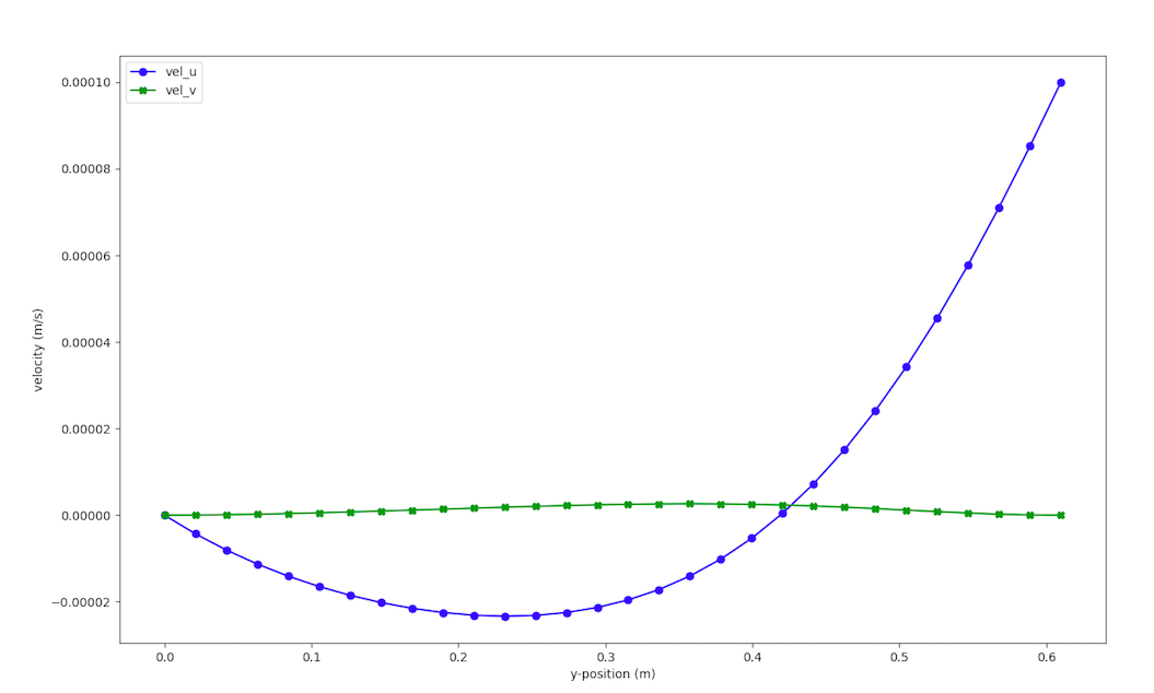 cavityprofile
For Re = 300
The flow output :
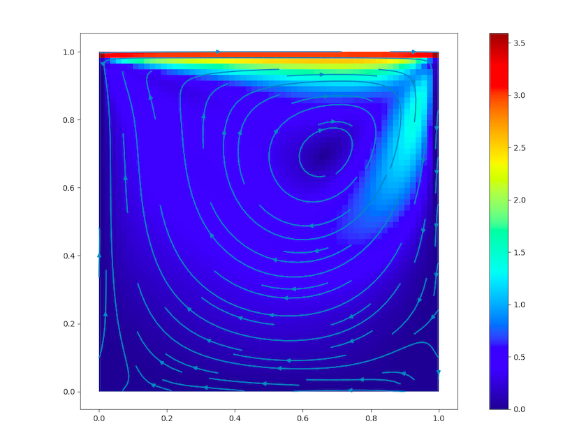 cavity300flow
The fields :
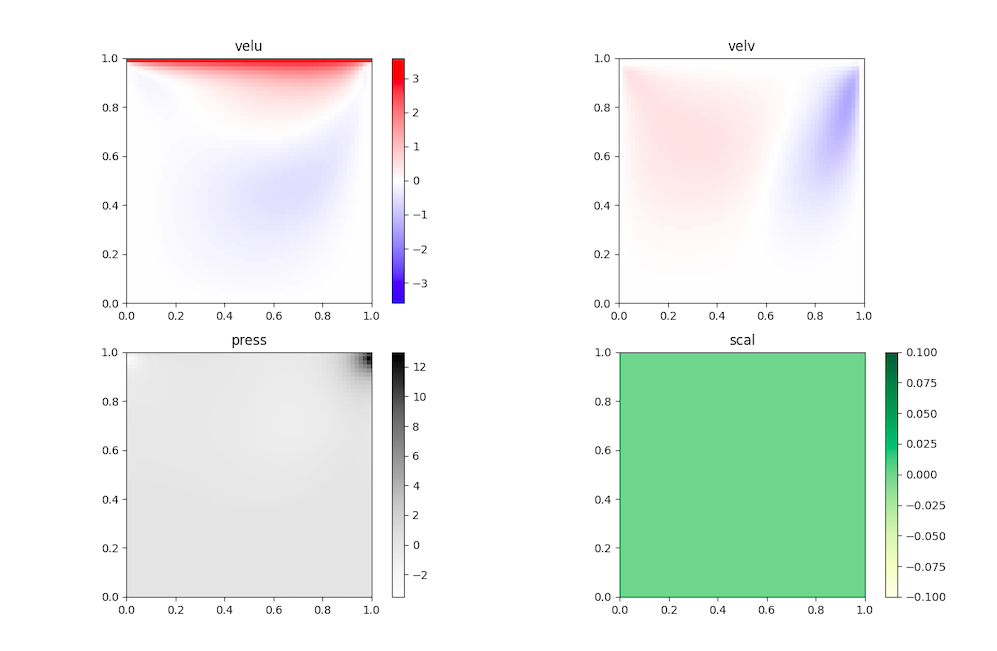 cavityfields300
The velocity profile :
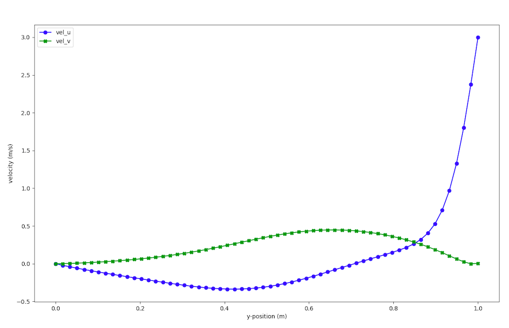 cavityeprofile300
Solver parameters:
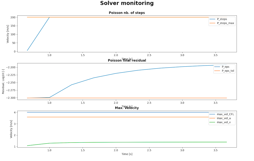 cavitysolver
Before modifications:
solver = NS_fd_2D_explicit(dom, obs_ib_factor=0.9, max_vel=2*vel)
To make the residual better we used a small delta_x and we manipulated the different parameters of the solver until having satisfactory results:
	  solver = NS_fd_2D_explicit(
	       dom, obs_ib_factor=0.01, press_maxsteps=200, press_tol=5.0e-3, max_vel=4.0)
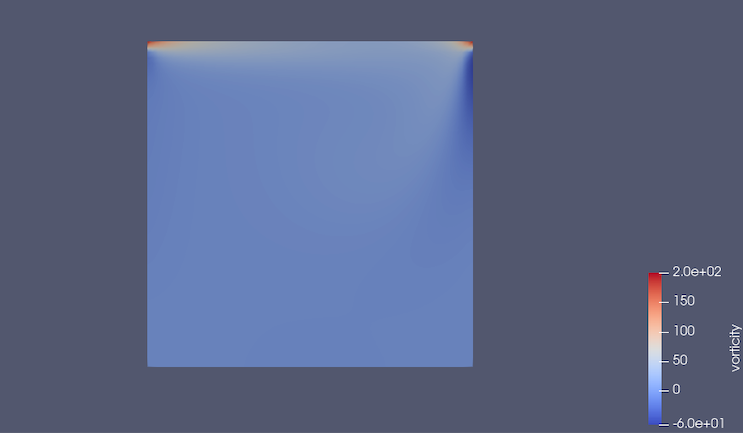 cavityVORTICITY
There is a high vorticity at the top corners, because they are singularities and the solver has difficulties to converge.
Comparison with the documentation for Re = 100
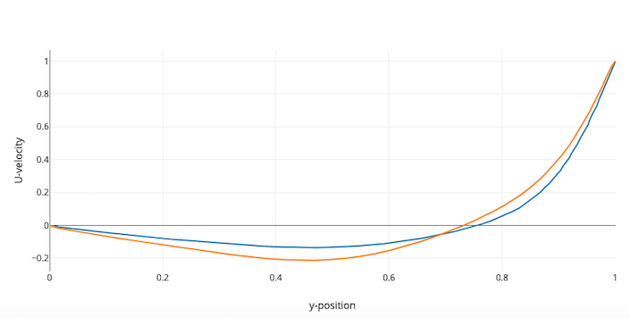 comparison
The curves are not exactly the same because the barbatruc solver is light weighted.
The blue curve is from the simulation and the orange curve is from the figure 5 (with AR=1) of the CFD SIMULATIONS OF LID DRIVEN CAVITY FLOW AT MODERATE REYNOLDS NUMBER, by Reyad Omari, Department of Mathematics, Al-Balqa Applied University, European Scientific Journal May 2013 edition vol.9, No.15 ISSN: 1857 – 7881 (Print) e - ISSN 1857- 7431 22
To have a better graph, one can try to:
- refine the mesh
- modify the pressure solver
Indeed, there are two main problems:
- the cavity has singularities
- there might be an issue of mass conservation, indeed the solver of Poisson did not converge enough and therefore mass conservation is not completely achieved