How to interact with barbatruc ?
LAUNCHING
To have the results :
Go to the folder where your file is :
cd folder/
To launch the simulation :
python3 cfd_cylinder.py
and you get :
	.  Rectangular Grid.
=======================

     y_max: 0.5m, nodes: 100
     +----------------------------+
     |                            |
     |                            |
     |                            |
     |                            |
     |                            |
     +----------------------------+
   (0,0)                        x_max: 1.0m, nodes: 200


                 periodic
     +----------------------------+
     |                            |
   inlet
     |                          outlet
     |                            |
     |                            |
     +----------------------------+
                  periodic

.  Fields stats
=======================
.  min|avg|max
 vel_u : 1.0 | 1.0 | 1.0
 vel_v : 0.1 | 0.10000000000000002 | 0.1
 scal : 0.0 | 0.0 | 0.0
 press : 0.0 | 0.0 | 0.0


===============================

  Iteration 1/200, Time :, 0.02s
  Reynolds : 111.92422560738474

.  Fields stats
=======================
.  min|avg|max
 vel_u : 0.12019082043493529 | 0.9940530128736734 | 1.3605910402433394
 vel_v : -0.3009720354811324 | 0.09675753736792093 | 0.4664584367055691
 scal : 0.0 | 0.0 | 0.0
 press : -2.2893733111942414 | 0.0 | 1.7798464788156056


===============================

  Iteration 2/200, Time :, 0.04s
  Reynolds : 112.09757332022016

.  Fields stats
=======================
.  min|avg|max
 vel_u : 0.023893464480471707 | 0.9953864667605914 | 1.3804213543256483
 vel_v : -0.329530409060508 | 0.0944418335727916 | 0.5040636022356708
 scal : 0.0 | 0.0 | 0.0
 press : -1.4163675489683598 | -7.105427357601002e-18 | 1.4278708080524152


===============================

  Iteration 3/200, Time :, 0.06s
  Reynolds : 111.90076036667641

.  Fields stats
=======================
.  min|avg|max
 vel_u : -0.06308165801559718 | 0.9935347780711958 | 1.3528315628913046
 vel_v : -0.3441370891819653 | 0.0922008027913569 | 0.5008225700261179
 scal : 0.0 | 0.0 | 0.0
 press : -1.276280378390031 | 2.1316282072803004e-18 | 1.2726099477265453


===============================
...
To interrupt the simulation :
ctrl + c
To know how much time the simulation takes :
time python3 cfd_cylinder.py


real	1m10.974s
user	1m49.836s
sys	0m14.051s
Remarks :
In the python file, a function is defined to compute the results :
def cfd_cylinder(nsave):
time_step is the observation time and not the one which respect the CFL.
nsave is the number of iteration :
time_step = t_end/nsave

t_end = 4.0 * lenght / vel
CHANGING CASE
Trick
Comment what you don’t want to use.
To change the solver :
 #solver = Lattice(dom, max_vel=2*vel)
 solver = NS_fd_2D_explicit(dom, obs_ib_factor=0.9)
obs_ ib _factor can be considered as a porosity factor of the obstacle (cylinder).
Take an example with known results, apply the two solvers, choose the one which is better for this case.
To change the boundary conditions :
dom.switch_bc_xmin_inlet(vel_u=vel)
#dom.switch_bc_xmax_outlet()
dom.switch_bc_ymax_wall_noslip()
dom.switch_bc_ymin_wall_noslip()
To change the case :
The default parameters are in fluid_domain.py. If they are specified in one of the examples (cfd_poiseuille.py, cfd_ lid _driven.py, cfd_cylinder.py) then those values are used.
Change the dimensions with delta_x = dimy/number of cells :
dom = DomainRectFluid(dimx=0.82, dimy=0.61, delta_x=0.02)
To have the Reynolds number that you want either change the velocity or the viscosity :
For Re = 20 and default viscosity nu_ = 1.0 :
vel = 32.7869
Be aware that by changing the velocity, you need to change the time : t_end = dimx/vel.
or with default velocity vel = 0.0001
dom = DomainRectFluid(dimx=0.82, dimy=0.61, delta_x=0.02, nu = 0.000003)
VIEWING
Results for a flow around a cylinder
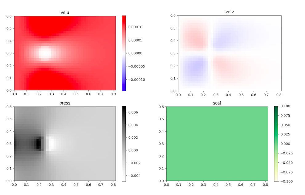
Fields at Small Reynolds Number :
dom.show_fields()
- vel_u : horizontal velocity
- vel_v : vertical velocity
- press : pressure
- scal : passive scalar which can simulate the trajectory of a leak of pollutant or the dissipation of a perfume in a room
 cylinderfields
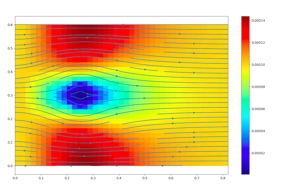
The flow output at Small Reynolds Number :
dom.show_flow()
- velocity field with its intensity (color code)
- streamlines (blue vectors)
 cylinderflow
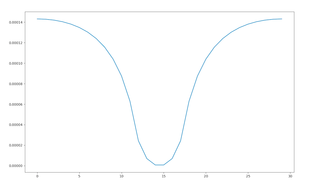
The velocity profile at Small Reynolds Number :
To get the profile at x=cste : change the value of xtgt.
dom.show_profile_y(xtgt=0.25, dimx=0.82, delta_x=0.02)
 cylinderprofile
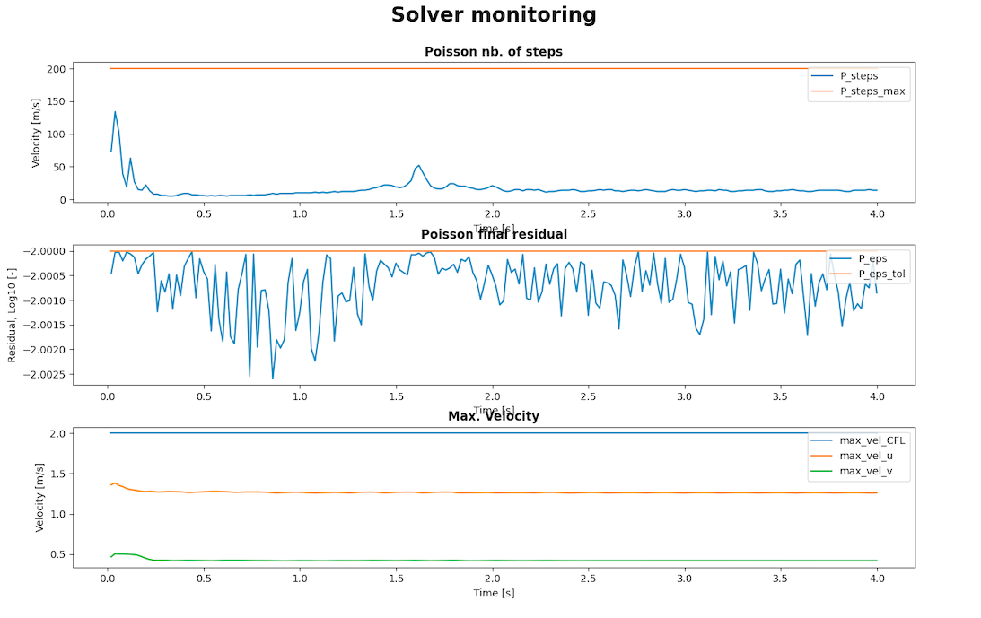
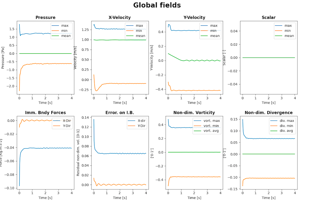
The monitors at High Reynolds Number :
This kind of monitoring only works with he Navier-Stokes solver; the LBM solver is not ready yet.
barbatruc monitor solver
The solver monitoring gives the following data in terms of time:
- the velocity for the number of step of Poisson
- the Poisson final residual
- the Maximum velocity
 karmanmonitor
barbatruc monitor glob
 karmanmonitor
The solver monitoring gives the following data in terms of time:
- pressure
- x-velocity
- y-velocity
- scalar
- Immersed boundaries forces, for further information
- Error on Immersed boundary
- Non dimensional Vorticity
- Non dimensional Divergence
Paraview
For the cylinder case, .xmf files are created and can be read with paraview. Those file are created in the time loop thanks to :
for i in range(nsave):
        dom.dump_paraview(time=time)
Open barbaresult.xmf in paraview :
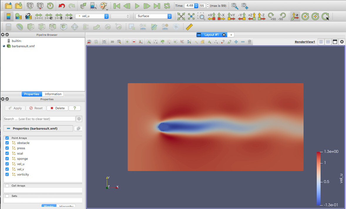 paraviewcylinder