Poiseuille Periodic 2D flow
1. Domain parameters
- Lx = dimx = 4 m
- Ly = width + d_x = 1.07 m
- delta_x = width/number of cells = 1/15 m
- U₀ = 1 m/s
- Re = 100, the most important parameter
To have great results : dimx must be at least twice dimy.
2. Boundary conditions
- Lower wall: no slip
- upper wall: no slip
- input: periodic
- output: periodic
A volumic force will be added to the flow.
Thanks to the Poiseuille equation, the source term is added as follow:
    dom.set_source_terms({
        "force_x": 8. * nu_ / width**2. * np.ones(dom.shape) * vel,
        "force_y": np.zeros(dom.shape),
        "scal": np.zeros(dom.shape)
    })
Reference case
the script
	"""Example on how to solve a Poiseuille problem  with the navier stokes solver"""

	import numpy as np
	import matplotlib.pyplot as plt
	from barbatruc.fluid_domain import DomainRectFluid
	from barbatruc.fd_ns_2d import NS_fd_2D_explicit
	#from barbatruc.lattice import Lattice

	__all__ = ["cfd_poiseuille"]


	# pylint: disable=duplicate-code
	def cfd_poiseuille(nsave):
	    """Startup computation
	    solve a poiseuille problem
	    """
	    width = 1.
	    length = width*4
	    dimx=length
	    vel = 1.0
	    t_end = 10.*length/vel
	    nu_ = 0.01
	    ncell = 15
	    d_x = width/ncell
	    dimy=width+d_x
	    delta_x=width/ncell
	    rho=1.12
	    dom = DomainRectFluid(
	        dimx=dimx,
	        dimy=dimy,
	        delta_x=delta_x,
	        nu_=nu_,
	        rho=rho)

	    dom.switch_bc_ymax_wall_noslip()
	    dom.switch_bc_ymin_wall_noslip()
	    dom.fields["vel_u"] += vel
	    dom.set_source_terms({
	        "force_x": 8. * nu_ / width**2. * np.ones(dom.shape) * vel,
	        "force_y": np.zeros(dom.shape),
	        "scal": np.zeros(dom.shape)
	    })

	    print(dom)
	    time = 0.0
	    time_step = t_end/nsave

	    #solver = Lattice(dom, max_vel=3*vel)
	    solver = NS_fd_2D_explicit(dom, max_vel=1.8)
	    for i in range(nsave):
	        time += time_step
	        solver.iteration(time, time_step)
	        print("\n\n===============================")
	        print(f"\n  Iteration {i+1}/{nsave}, Time :, {time}s")
	        print(f"  Reynolds : {dom.reynolds(width)}")
	        print(dom.fields_stats())
	        dom.dump_paraview(time=time)
	        dom.dump_global(time=time)

	    y = np.linspace(0,1.07,num=1000)
	    u=np.zeros(len(y))
	    u_bulk=0.66
	    Umax=(3/2)*u_bulk

	    for i in range(len(y)):
	        u[i]=Umax*4*(y[i]/dimy)*(1-(y[i]/dimy))
	    plt.plot(y,u,color="red",marker="", label= 'theoretical curve')

	    dom.show_profile_y()
	    solver.plot_monitor()
	    dom.show_fields()
	    dom.show_flow()
	    dom.show_debit_over_x()

	    print('Normal end of execution.')


	if __name__ == "__main__":
	    cfd_poiseuille(10)
The flow output :
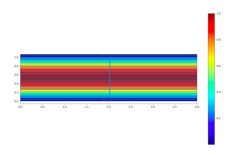 poiseuilleflow
The fields :
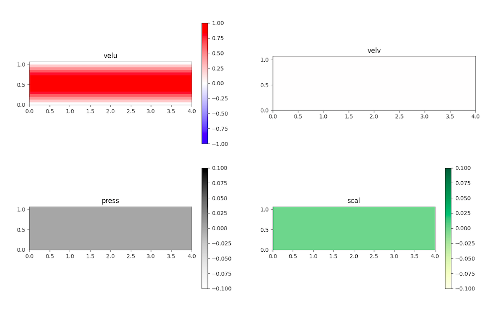 poiseuillefields
The flow velocity profile :
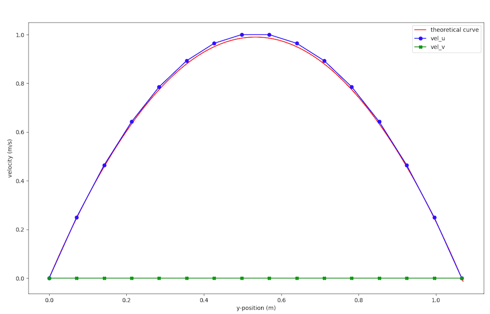 poiseuilleprofile
`
poiseuilleprofile
`
Global parameters:
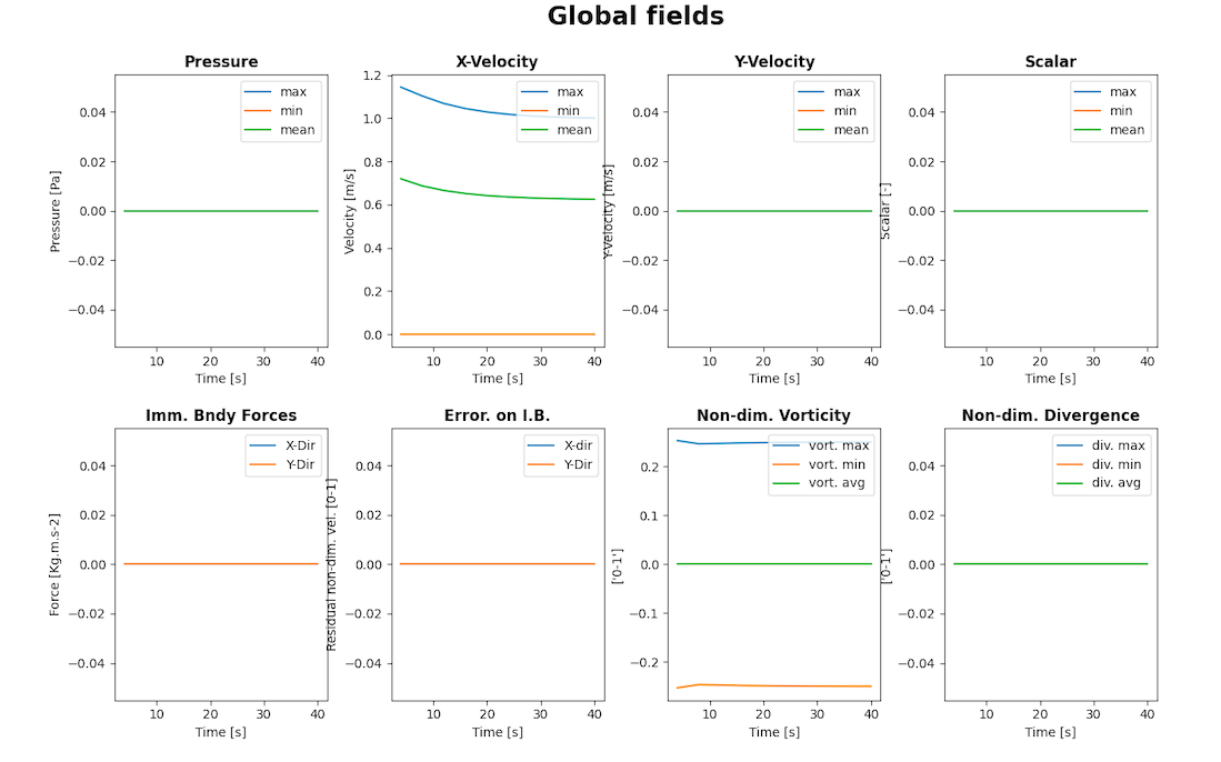 poiseuilleglob
We added a volumic force to simulate the pressure gradient, therefore, the solution correspond to the analytic solution:
Pmax = Pmin = Pmean = 0
You can obtain the mean velocity from the X-Velocity graph.
Solver parameters:
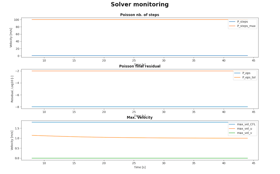 poiseuillesolver
max_vel is a parameter of the solver, one can study the convergence of the simulation thanks to the residual of Poisson.
For instance, using max_vel=1.8 instead of max_vel=2.0 improves the residual:
solver = NS_fd_2D_explicit(dom, max_vel=1.8)
To go further: how to modify the parameters to get Re = 19
Change the value of the viscosity to obtain the correct value of the Reynolds number by keeping the default parameters
 dom = DomainRectFluid(nu_=0.0000032105, dimx=0.82, dimy=0.61, delta_x=0.02)

 vel = 0.0001
Put the value of the initial velocity that you want and adapt the viscosity to have the right Reynolds number
 dom = DomainRectFluid(nu_=0.048158, dimx=0.82, dimy=0.61, delta_x=0.02)

 vel = 1.5
Modify the dimensions of the problem
 dom = DomainRectFluid(nu_=0.000015789,dimx=0.006, dimy=0.0002,delta_x=0.00001)

 vel=1.5
Pay attention to the value of the number of convective times : Lx/U₀=t_end